Feature scaling and transformation in machine learning

In this tutorial we will learn how to scale or transform the features using different techniques.

import pandas as pd
import numpy as np
import matplotlib.pyplot as plt

diabetes=pd.read_csv('diabetes_cleaned.csv')

features_df= diabetes.drop('Outcome',axis = 1)
target_df=diabetes['Outcome']

features_df.describe()

	Pregnancies	Glucose	BloodPressure	SkinThickness	Insulin	BMI	DiabetesPedigreeFunction	Age
count	768.000000	768.000000	768.000000	768.000000	768.000000	768.000000	768.000000	768.000000
mean	3.845052	121.539062	72.405184	29.108073	152.222767	32.307682	0.471876	33.240885
std	3.369578	30.490660	12.096346	8.791221	97.387162	6.986674	0.331329	11.760232
min	0.000000	44.000000	24.000000	7.000000	-17.757186	18.200000	0.078000	21.000000
25%	1.000000	99.000000	64.000000	25.000000	89.647494	27.300000	0.243750	24.000000
50%	3.000000	117.000000	72.202592	29.000000	130.000000	32.000000	0.372500	29.000000
75%	6.000000	140.250000	80.000000	32.000000	188.448695	36.600000	0.626250	41.000000
max	17.000000	199.000000	122.000000	99.000000	846.000000	67.100000	2.420000	81.000000

As you can see range of columns are very high for e.g. Age range is 21-81. ML models always give you better result when all of the features are in same range. So let’s do that using various techniques.

Feature Scaling and Standardization

When all features are in different range then we change the range of those features to a specific scale ,this method is called feature scaling.

• Normalization and Standardization are two specific Feature Scaling methods.

Min Max Scaler

from sklearn.preprocessing import MinMaxScaler

scaler=MinMaxScaler(feature_range=(0,1))
rescaled_features=scaler.fit_transform(features_df)
rescaled_features

array([[0.35294118, 0.67096774, 0.48979592, ..., 0.31492843, 0.23441503,
        0.48333333],
       [0.05882353, 0.26451613, 0.42857143, ..., 0.17177914, 0.11656704,
        0.16666667],
       [0.47058824, 0.89677419, 0.40816327, ..., 0.10429448, 0.25362938,
        0.18333333],
       ...,
       [0.29411765, 0.49677419, 0.48979592, ..., 0.16359918, 0.07130658,
        0.15      ],
       [0.05882353, 0.52903226, 0.36734694, ..., 0.24335378, 0.11571307,
        0.43333333],
       [0.05882353, 0.31612903, 0.46938776, ..., 0.24948875, 0.10119556,
        0.03333333]])

rescaled_diabetes = pd.DataFrame(rescaled_features, columns=features_df.columns)
rescaled_diabetes

	Pregnancies	Glucose	BloodPressure	SkinThickness	Insulin	BMI	DiabetesPedigreeFunction	Age
0	0.352941	0.670968	0.489796	0.304348	0.274029	0.314928	0.234415	0.483333
1	0.058824	0.264516	0.428571	0.239130	0.101819	0.171779	0.116567	0.166667
2	0.470588	0.896774	0.408163	0.239130	0.333110	0.104294	0.253629	0.183333
3	0.058824	0.290323	0.428571	0.173913	0.129385	0.202454	0.038002	0.000000
4	0.000000	0.600000	0.163265	0.304348	0.215057	0.509202	0.943638	0.200000
...	...	...	...	...	...	...	...	...
763	0.588235	0.367742	0.530612	0.445652	0.228950	0.300613	0.039710	0.700000
764	0.117647	0.503226	0.469388	0.217391	0.204424	0.380368	0.111870	0.100000
765	0.294118	0.496774	0.489796	0.173913	0.150224	0.163599	0.071307	0.150000
766	0.058824	0.529032	0.367347	0.239130	0.221796	0.243354	0.115713	0.433333
767	0.058824	0.316129	0.469388	0.260870	0.121509	0.249489	0.101196	0.033333

768 rows × 8 columns

rescaled_diabetes.boxplot(figsize=(12,10),rot=45)

<matplotlib.axes._subplots.AxesSubplot at 0x164058b0>

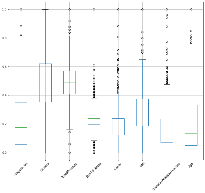
You can see all the data column’s range is between 0-1 now.

But here is one Catch!! MinMaxScaler is very sensitive to your data so make sure your whole prediction should not be hampered , like in this case if you see it has change age’s min to 0 but that is not the one we are looking for.

Standardization

Standardization is applied on feature wise , we calculate the mean of each feature then subtract each feature value from the mean and then divide it with the standard deivation Standardization centers mean of all our numeric features at 0 and expresses each value of the feature by the multiples of the std dev.

This is usually preferred because it is less outlier sensitive.

from sklearn.preprocessing import StandardScaler

scaler=StandardScaler()
standardized_features=scaler.fit_transform(features_df)

standardized_diabetes = pd.DataFrame(standardized_features, columns=features_df.columns)
standardized_diabetes

	Pregnancies	Glucose	BloodPressure	SkinThickness	Insulin	BMI	DiabetesPedigreeFunction	Age
0	0.639947	0.868403	-0.033518	0.670643	0.685496	0.185089	0.468492	1.425995
1	-0.844885	-1.199150	-0.529859	-0.012301	-0.842893	-0.817471	-0.365061	-0.190672
2	1.233880	2.017044	-0.695306	-0.012301	1.209840	-1.290106	0.604397	-0.105584
3	-0.844885	-1.067877	-0.529859	-0.695245	-0.598238	-0.602636	-0.920763	-1.041549
4	-1.141852	0.507402	-2.680669	0.670643	0.162111	1.545707	5.484909	-0.020496
...	...	...	...	...	...	...	...	...
763	1.827813	-0.674057	0.297376	2.150354	0.285411	0.084833	-0.908682	2.532136
764	-0.547919	0.015127	-0.198965	-0.239949	0.067744	0.643403	-0.398282	-0.531023
765	0.342981	-0.017691	-0.033518	-0.695245	-0.413288	-0.874760	-0.685193	-0.275760
766	-0.844885	0.146400	-1.026200	-0.012301	0.221915	-0.316191	-0.371101	1.170732
767	-0.844885	-0.936604	-0.198965	0.215347	-0.668142	-0.273224	-0.473785	-0.871374

768 rows × 8 columns

standardized_diabetes.boxplot(figsize=(12,10),rot=45)

<matplotlib.axes._subplots.AxesSubplot at 0x1679ec30>

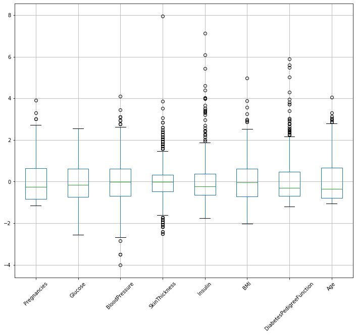
You can see that all features’ mean have been centered to zero and if any feature is not having many outliers then its median should not be far away from the mean.

Normalization

Normalization converts the feature vectors to their unit norm representations , there are different types of unit norms such as

1. L1 Normalization
2. L2 Normalization
3. Max Normalization

This is not useful with data having outliers!

from sklearn.preprocessing import Normalizer

L1 Normailization

normalizer = Normalizer(norm='l1')
l1_normalized_features = normalizer.fit_transform(features_df)

l1_normalized_diabetes = pd.DataFrame(l1_normalized_features, columns=features_df.columns)
l1_normalized_diabetes.head()

	Pregnancies	Glucose	BloodPressure	SkinThickness	Insulin	BMI	DiabetesPedigreeFunction	Age
0	0.010635	0.262335	0.127622	0.062039	0.388074	0.059557	0.001111	0.088627
1	0.003235	0.274956	0.213495	0.093809	0.227047	0.086045	0.001135	0.100278
2	0.013116	0.300029	0.104928	0.047546	0.442615	0.038200	0.001102	0.052464
3	0.003103	0.276169	0.204799	0.071369	0.291684	0.087195	0.000518	0.065163
4	0.000000	0.298873	0.087262	0.076355	0.366502	0.094025	0.004991	0.071991

l1_normalized_diabetes.iloc[0]

Pregnancies                 0.010635
Glucose                     0.262335
BloodPressure               0.127622
SkinThickness               0.062039
Insulin                     0.388074
BMI                         0.059557
DiabetesPedigreeFunction    0.001111
Age                         0.088627
Name: 0, dtype: float64

Every row in your dataset is a feature vector and normalization is a technique to convert those feature vector by their unit magnitude there are different types of unit magnitudes here we have converted using L1 unit magnitude.

In L1 normalization summation of absolute values of these normalized features is 1.

l1_normalized_diabetes.iloc[0].abs().sum()

1.0

L2 Normalization

In L2 normalization every feature vector or records in your dataset will be converted to their L2 unit magnitude and sum of the individual features’ square will be 1

normalizer = Normalizer(norm='l2')
l2_normalized_features = normalizer.fit_transform(features_df)
l2_normalized_diabetes = pd.DataFrame(l2_normalized_features, columns=features_df.columns)
l2_normalized_diabetes.head()

	Pregnancies	Glucose	BloodPressure	SkinThickness	Insulin	BMI	DiabetesPedigreeFunction	Age
0	0.021225	0.523547	0.254698	0.123812	0.774487	0.118859	0.002218	0.176874
1	0.007251	0.616359	0.478585	0.210287	0.508963	0.192884	0.002545	0.224790
2	0.023805	0.544535	0.190439	0.086292	0.803320	0.069332	0.002000	0.095219
3	0.006612	0.588467	0.436392	0.152076	0.621527	0.185797	0.001104	0.138852
4	0.000000	0.596386	0.174127	0.152361	0.731335	0.187622	0.009960	0.143655

l2_normalized_diabetes.iloc[0].pow(2).sum()

0.9999999999999997

Maximum Normalization

Now let’s talk about Maximum normalization here the maximum value of a feature vector is converted to 1 and other values of that feature vector will be converted in terms of this maximum.

normalizer = Normalizer(norm='max')
max_normalized_features = normalizer.fit_transform(features_df)
print(type(max_normalized_features))
max_normalized_diabetes = pd.DataFrame(max_normalized_features, columns=features_df.columns)
max_normalized_diabetes.head()

<class 'numpy.ndarray'>

	Pregnancies	Glucose	BloodPressure	SkinThickness	Insulin	BMI	DiabetesPedigreeFunction	Age
0	0.027405	0.675991	0.328861	0.159863	1.000000	0.153468	0.002864	0.228375
1	0.011765	1.000000	0.776471	0.341176	0.825756	0.312941	0.004129	0.364706
2	0.029633	0.677856	0.237064	0.107420	1.000000	0.086306	0.002489	0.118532
3	0.010638	0.946809	0.702128	0.244681	1.000000	0.298936	0.001777	0.223404
4	0.000000	0.815476	0.238095	0.208333	1.000000	0.256548	0.013619	0.196429

if you look at the above df you can see one feature in every record is transformed into 1 and other features are represented in terms of this max.

Binarizer

Now sometimes it may be required that we would want to discretize our numerical features there we can use binarizer. In binarizer we provide a threshold value for each feature and it will convert all values which is less than the threshold to zero and all values which is greater than the threshold to 1.

scaler=Binarizer(threshold=float((features_df[['Pregnancies']]).mean()))
binarized_features=scaler.fit_transform(features_df[['Pregnancies']])

from sklearn.preprocessing import Binarizer
for i in range(1,features_df.shape[1]):
    scaler=Binarizer(threshold=float(features_df[features_df.columns[i]].mean())). \
                                    fit(features_df[[features_df.columns[i]]])
    new_binarized_feature = scaler.transform(features_df[[features_df.columns[i]]])
    binarized_features = np.concatenate((binarized_features,new_binarized_feature),axis=1)

binarized_diabetes = pd.DataFrame(binarized_features, columns=features_df.columns)
binarized_diabetes.head(20)

	Pregnancies	Glucose	BloodPressure	SkinThickness	Insulin	BMI	DiabetesPedigreeFunction	Age
0	1.0	1.0	0.0	1.0	1.0	1.0	1.0	1.0
1	0.0	0.0	0.0	0.0	0.0	0.0	0.0	0.0
2	1.0	1.0	0.0	0.0	1.0	0.0	1.0	0.0
3	0.0	0.0	0.0	0.0	0.0	0.0	0.0	0.0
4	0.0	1.0	0.0	1.0	1.0	1.0	1.0	0.0
5	1.0	0.0	1.0	0.0	0.0	0.0	0.0	0.0
6	0.0	0.0	0.0	1.0	0.0	0.0	0.0	0.0
7	1.0	0.0	1.0	0.0	0.0	1.0	0.0	0.0
8	0.0	1.0	0.0	1.0	1.0	0.0	0.0	1.0
9	1.0	1.0	1.0	0.0	0.0	0.0	0.0	1.0
10	1.0	0.0	1.0	0.0	0.0	1.0	0.0	0.0
11	1.0	1.0	1.0	0.0	1.0	1.0	1.0	1.0
12	1.0	1.0	1.0	0.0	1.0	0.0	1.0	1.0
13	0.0	1.0	0.0	0.0	1.0	0.0	0.0	1.0
14	1.0	1.0	0.0	0.0	1.0	0.0	1.0	1.0
15	1.0	0.0	1.0	0.0	0.0	0.0	1.0	0.0
16	0.0	0.0	1.0	1.0	1.0	1.0	1.0	0.0
17	1.0	0.0	1.0	0.0	0.0	0.0	0.0	0.0
18	0.0	0.0	0.0	1.0	0.0	1.0	0.0	0.0
19	0.0	0.0	0.0	1.0	0.0	1.0	1.0	0.0

You can see all vectors have been represented using zero or 1 Now that we have transformed our data using different techniques let’s do some classification now.

Now lets build a classification model and see the differences:

from sklearn.linear_model import LogisticRegression
from sklearn.model_selection import train_test_split
from sklearn.metrics import accuracy_score

def buildmodel(X,Y,test_frac):
    x_train,x_test,y_train,y_test =train_test_split(X,Y,test_size=test_frac)
    model =LogisticRegression(solver='liblinear').fit(x_train,y_train)
    y_pred=model.predict(x_test)
    print('Accuracy of the model is',accuracy_score(y_test,y_pred))

buildmodel(rescaled_diabetes,target_df,test_frac=.2)#using MinMaxScaler

Accuracy of the model is 0.7857142857142857

buildmodel(standardized_diabetes,target_df,test_frac=.2)#using StandardScaler

Accuracy of the model is 0.7662337662337663

buildmodel(l1_normalized_features,target_df,test_frac=.2)

Accuracy of the model is 0.6103896103896104

buildmodel(l2_normalized_features,target_df,test_frac=.2)

Accuracy of the model is 0.6623376623376623

buildmodel(max_normalized_features,target_df,test_frac=.2)

Accuracy of the model is 0.7337662337662337

buildmodel(binarized_features,target_df,test_frac=.2)

Accuracy of the model is 0.6753246753246753

You can get the notebook used in this tutorial here and dataset used here

Thanks for reading!